Full Text

1. Introduction

In India, the coronavirus disease 2019 (COVID-19) is the global pandemic of coronavirus share caused by severe acute respiratory syndrome coronavirus 2 (SARS-CoV-2). The first observed case of COVID-19 in India was initiated from China on January 30, 2020. This virus has spread rapidly across the whole country, especially Maharashtra with the highest confirmed cases of 107958 (June 15, 2020). COVID -19 has a significant correlation with air quality, average, and minimum temperature [1]. The two transmission mode of corona is respiratory and contact. The sanitation and hygienic environments are crucial to protect human health during this infectious COVID-19 outbreak. Ensuring decent and frequent hand wash practices in communities, homes, and health care will help prevent and reduce man-to-man transmission of the COVID-19 virus was avowed by World Health Organization (WHO) [2]. The physical examination of the patients was found to have dry mucous membranes, difficulty breathing, sore throat, headache, or cough [3]. All these lead to a lockdown of many countries, including India from March 25, 2020, to May 31, 2020, in four phases. In few areas of containment zone, the lockdown is extended up to June 30, 2020, as fifth phase. In this study, the spatial data i.e confirmed cases and testing samples, are focused. The confirmed cases are focused on understanding the rate of increase per day in every state and thereby in India. Also, the testing sample per day in every state is examined.

Few studies on geographical weighted regression (GWR) were explored for this study, and implemented on Indian COVID-19 data. Mollalo for COVID-19 data in the US has performed different models on the dataset, which included thirty-five environmental variables, socioeconomic, behavioral, topographic and demographic factors. The five different models used were three global models, namely ordinary least square (OLS), SLM and SEM, and two local models, namely GWR and multiscale GWR (MGWR). The results of MGWR achieved the highest goodness-of-fit with the most parsimonious model compared to others. The spatial variability of MGWR in different countries can reflect different behavior of COVID-19 cases in response to the explanatory variables [4].

Wang performed GWR to examine the relationship between the index of frequency of extreme precipitation and other climatic extreme indices in China that includes the frequency of warm days, warm nights, cold days, and cold nights. Based on statistical tests, the regression relationship was observed to be significant between spatial non-stationarity and explanatory variables that exhibited significant spatial inconsistency. GWR was implemented in a case of ecological inference to solve the problems related to the inference of the individual [5]. Calvo & Escolar proposed GWR approach for solving complications of spatial aggregation bias and spatial autocorrelation that affect all well-known approaches of ecological inference. This estimation process can theoretically and intuitively compute, showing that GWR approach to Goodman and King’s Ecological Inference methods results in unbiased and consistent local estimates of ecological data that reveal extreme spatial heterogeneity [6]. GWR on data of house price varying with both power and rotation parameters to generate different Minkowski distances, the study proved that the local collinearity can be both negatively and positively affected by distance metric choice. The results indicate that distance metric choice can provide a useful extra tuning component to address local collinearity issues in spatially varying coefficient modelling and helps to understand the interaction of distance metric and collinearity can provide insight into the nature and structure of the data relationships [7].

Franch-Pardo carried out an assessment of sixty three scientific articles on geospatial and spatial-statistical analysis of COVID-19. The study is grouped into the categories of disease mapping: spatiotemporal analysis, health and social geography, environmental variables, data mining, and web-based mapping. It was clarified that the spatiotemporal dynamics of COVID-19 needs very strong decision making, planning and community action. Also, it emphasized that the challenges from an interdisciplinary perspective with proactive planning, international solidarity and a global perspective needs to be addressed to fight COVID-19 [8]. Gupta used long-term climatic data of air temperature (V1), rainfall (V1), actual evapotranspiration (V1), solar radiation (V1), specific humidity, wind speed with topographic altitude and density of population at the regional point to examine the spatial association with the quantity of COVID-19 infections. Their results proved Variable Importance of Projection through PLS technique that had very higher significance over all V1’s [9].

Boulos & Geraghty (2020) discusses about the disease mapping and the social media reactions for disease spread, predictive risk mapping using population travel data, tracing and mapping super-spreader trajectories and contacts across space and time. The study is how GIS and mapping dashboards can support the fight against infectious disease outbreaks and epidemics [10]. Krishnakumar & Rana gives good insights to make effective approach to culminate the world threat COVID-19 in India [11]. Pulla (2020) expresses that the transmission of COVID-19 by asymptomatic people would reduce the effectiveness of airport screening and quarantine measures. It was communicated that India would have confirmed cases of COVID-19 between around 100 000 and 1.3 million by the middle of May if the virus continues to spread at its current rate [12].

2. Data and methodology

The study includes the spatial models, namely ordinary least square (OLS), geographical weighted regression (GWR), and generalized linear regression (GLR). The details of each models is discussed in Spatial Regression Models section. The day to day data was collected from Ministry of health and family welfare (Table 1) and analyzed using ArcGIS Pro with spatial models. The samples for testing data for state-wise and all over India were obtained from Statista and ICMR websites. The testing data were found to vary based on testing labs available in each state. Total number of samples tested as on June 15, 2020 in few states such as TN (729002), MH (671348), RJ (609296) and AP (567375) were updated when compared with the confirmed cases in TN (44661), MH (107958), RJ (12694) and AP (6163). The time series graph for day wise increase in India and twelve different states was obtained using STATA 12 IC. The two way graph for sample tested and confirmed case for states was performed on STATA 12 IC. The study includes the increase of COVID-19 confirmed cases after the lockdown period and is analyzed using ArcGIS on the confirmed case of June 15, 2020 as the response variable with the explanatory variables of COVID-19 cases i.e. March 15, 2020, April 7, April 12, May 12 and June 1, 2020. Here, for this study, the confirmed cases of dataset is classified into three cases ie. case-1: June 15, 2020 Vs March 15 and April 7, 2020; case-2: June 15, 2020 Vs April 12, May 12 and June 1, 2020; and case-3: June 15, 2020 Vs March 15, April 7, April 12, May 12 and June 1, 2020.

2.1 Spatial regression models

2.1.1 Ordinary least square

Ward & Gleditsch discusses about OLS as a linear regression approach that examines the relationships between dependent variable and a set of explanatory variables and is represented with the following notation (eq. 1)

y_i=β₀+x_i β+ ϵ_i ------------------ (1)

where i represents any country, y_i is the confirmed cases (dependent variable), the intercept of the model (β₀), the vector of selected explanatory variables (x_i), the vector of regression coefficients (β), and random error term (ε_i) [13]. Based on the nature of the spatial dependence, OLS will be either incompetent with incorrect standard errors or biased and inconsistent [14]. If spatial dependence among the data exists, then it violates assumptions about the error term [15, 16].

2.1.2 Generalized linear regression

GLR is a regression model used to generate predictions or to model a dependent variable in relation to a set of explanatory variables. Its prediction can be used to examine and quantifies relationships among features. The tool is used to fit continuous (OLS), binary (logistic), and count (Poisson) models. A count model assumes that the mean and variance of the dependent variable are equal, and moreover, the values of the dependent variable cannot be negative or contain decimals. The notation of GLR is as follows in eq. 2.

y= β₀+ β₁ x₁ + β₂ x₂+⋯+ β_n x_n + e₁ ------------ (2)

where β₀ is the intercept, β₁, and β₂ are the slope and coefficient of the explanatory variables in regressions with x₁ x₂ and, …x_n, respectively. The term ei is the error terms, and y is the dependent variable [17].

Table 1: Covid- 19 data as on June 15, 2020.

2.1.3 Geographically weighted regression

GWR is a spatial techniques mostly used in geography and many other disciplines. GWR is a local model of the variable to predict by fitting a regression equation to each feature in the dataset. It should be noted that GWR is not an appropriate method for small datasets and does not work with multipoint data. The notation of GWR is given in eq. 3 [4].

--- (3)

where i is a country, yi is the value for the confirm cases, the intercept (β_i0), the jth regression parameter (β_ij), X_ij is the value of the jth explanatory parameter, and εi is a random error term.

3. Findings and results

The models are generated on the datasets obtained from https://www.mohfw.gov.in/ and the analysis was performed on ArcGIS Pro. The results of OLS model (Figure 1) summaries the coefficient, T-statistic and P-value along with VIFs on explanatory variables assumed (Tables 2, 3 and 4); the selected variables have relatively low multi-collinearity since the Variance Inflation Factor (VIFs) for all of explanatory variables were positively associated with confirmed cases (p< 0.01). The p-value for Con-June-1 (0.0000) is much better with VIF (66.16) over the other explanatory in case-1, similarly in case-II, p-value of Con-Apr-7(0.00001) is good fit; and Con-June-1 (0.0000) in case-III.

Table 2: Summary of OLS model on explanatory variables –Case-1.

Table 3: Summary of OLS model on explanatory variables – Case –II.

Table 4: Summary of OLS model on explanatory variables – Case –III.

GLR model (Figure 2) with the summary of the three different models is shown in the Tables 5, 6 and 7. The z-score for the intercept is 1720.1645, Con-Mar-15 (-28.6294), Con-Apr-7 (58.2404), Con-Apr-12 (52.3568), Con-Mar-12 (166.8258) and Con-June-1 (-143.532) in table 5. Z-scores are standard deviations. Both z-scores and p-values are associated with the standard normal distribution. In table 6 the z-score for intercept (2199.1819), Con-Mar-15 (51.5807), and Con-Apr-7 (575.7223) and in table 7, the z-score for intercept (1769.2154), Con-Apr-12 (359.7744), Con-May-12 (168.4036), and Con-June-1 (-180.429).

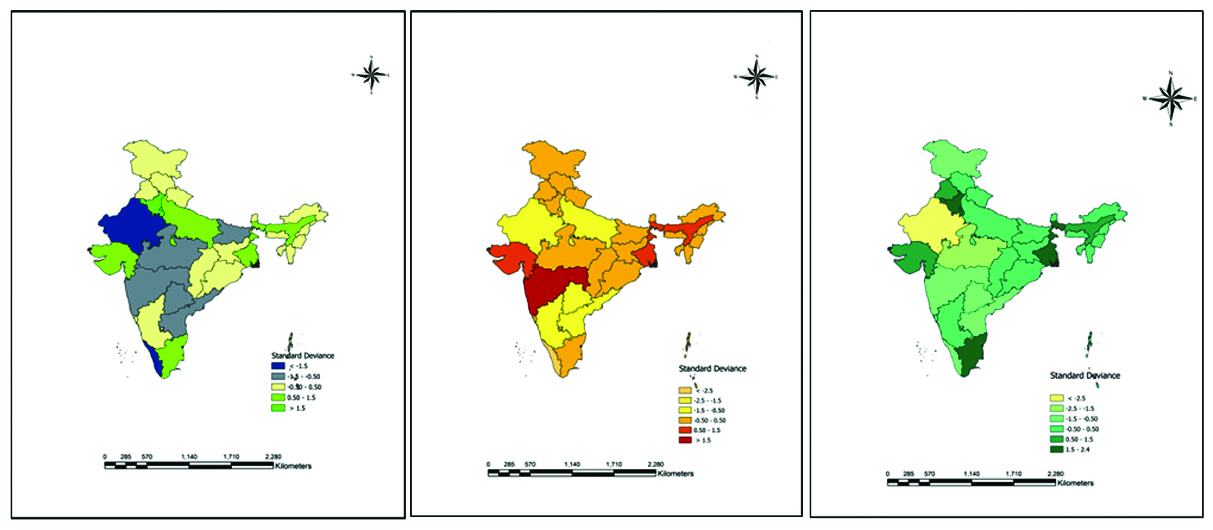
Figure 1: OLS model for confirmed cases in India.

Table 5: Summary of GLR model on explanatory variables – Case-I.

Table 6: Summary of GLR model on explanatory variables –Case-II.

Table 7: Summary of GLR model on explanatory variables –Case-III.

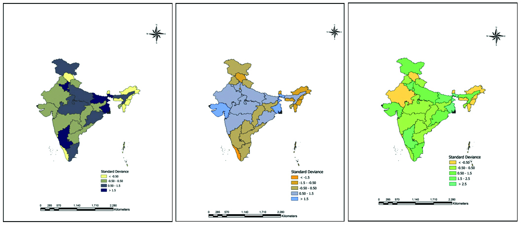
Figure 2: GLR model for confirmed cases in India.

GWR model (Figure 3) with the summary of the three different models (Tables 8, 9 and 10); the model is described based on the various factors such as Sigma square and Sigma Square MLE and DF. Finally, sigma-squared is used for AICc computations. From the tables obtained R2 (0.9983) in Case-I is much closer to 1 over other cases i.e, R² (0.7804) in Case-II and R² (0.9939) in Case-III. And based on AICc and R² values, the model is coined as better model [18].

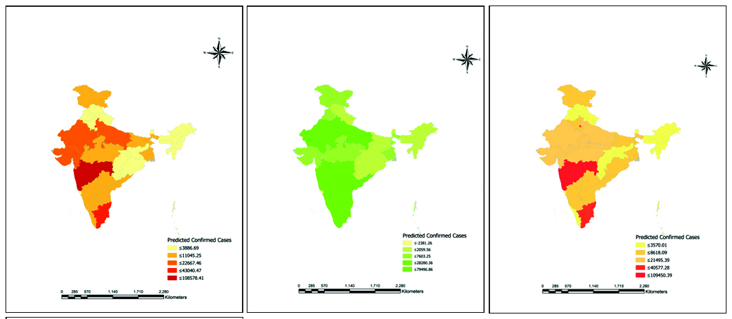
Figure 3: GWR model for confirmed cases in India.

Table 8: Summary of GWR model on explanatory variables –Case-I.

Sigma-Sq.

644959.6972

Table 9: Summary of GWR model on explanatory variables –Case-II.

Sigma-Sq.

Table 10: Summary of GWR model on explanatory variables –Case-III.

Sigma-Sq.

The relationship charts (Figure 4, 5 and 6) between variables ie dependent and explanatory. The R-squared obtained (Figure 4) GLR (R² = 0.99) and GWR (R² = 0.9983) similarly (Figure 5) GLR (R² = 0.68) and GWR (R2 = 0.7804) and (Figure 6) GLR (R² = 0.99) and GWR (R² = 0.9939) respectively. Deviance residual chart for GLR and GWR is shown in Figure 7, 8 and 9.

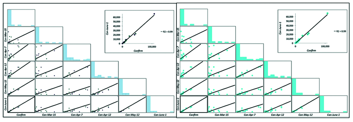
Figure 4: Case- I- Relationships graph of GLR (Left) and GWR (Right).

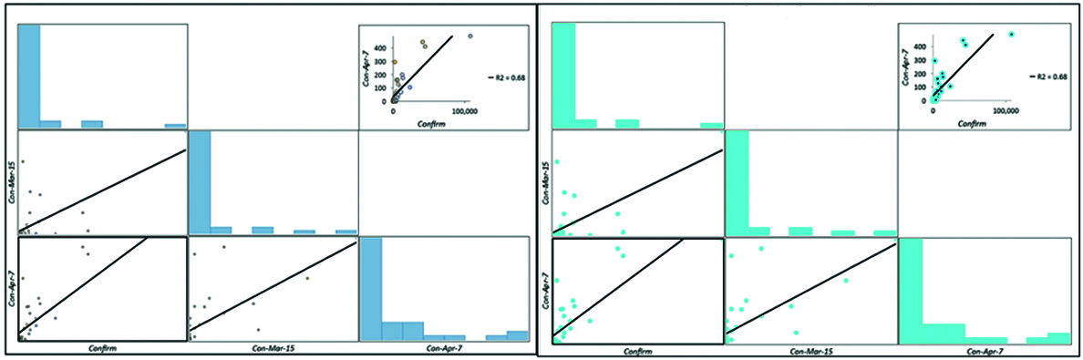
Figure 5: Case- II- Relationships graph of GLR (Left) and GWR (Right).

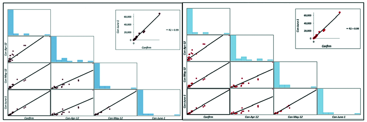
Figure 6: Case- III -Relationships graph of GLR (Left) and GWR (Right).

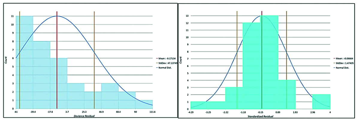
Figure 7: Case- I- Distribution of Deviance Residual graph for GLR (Left) and GWR (Right).

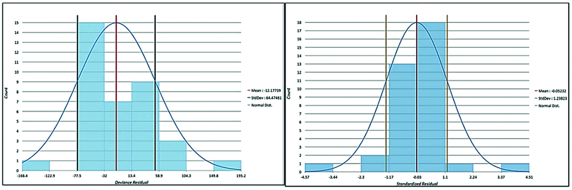
Figure 8: Case- II- Distribution of Deviance Residual graph for GLR (left) and GWR (Right).

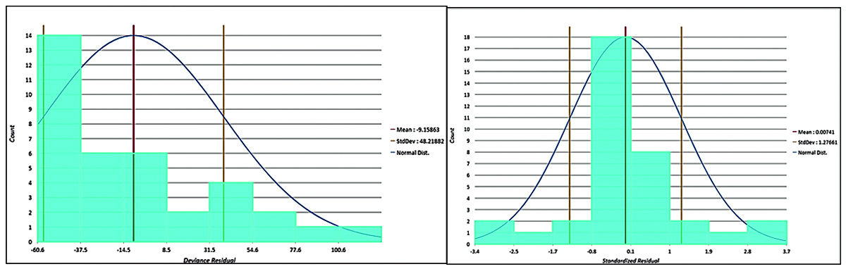
Figure 9: Case- III- Distribution of Deviance Residual graph for GLR (left) and GWR (Right).

On comparing the three models (Table 11) the values of AICc and Adj R2, implies that the measure of model performance of regression models can be understood with AICs value. The model with the lower AICc value provides a better fit to the observed data. On examining table 11, GWR model (618.9038) is better over GLR (81132) and OLS (641.192). Adj R-sq value varies from 0.0 to 1.0 and Adj-R-sq of GWR is much nearer to 1 compared to OLS and GLR model. Hence, GWR model is the better fit model for the COVID-19 data in this study.

Table 11: Measure of model fit/ performance for OLS, GWR and GLR in modelling of COVID-19 confirm cases in India.

The predicted values of GWR for Case -1 (Table 12), FIDs – 18 (MH) with predicted values is 108578.4, similarly FID -17 (MP) has predicted cases (11045.25), FID – 23 (DL) with cases (39150.27), FID – 28 (TN) with 43040.47 and FID- 29 (TS) with cases (6228.23). The following equation y = 0.09130 + -0.00002 x and R2 = 0.05487770288 was generated for case –I.

Table 12: Summary table of GWR predicted model with explanatory variables –Case-I.

Daywise increase in states Figure 10 represents the graphs for 12 different states with MH and TN having maximum cases and the states, namely KL and KA where the curve is flattened. The graphs indicate the day wise increase in the number of confirm cases. Figure 11a represents each curve for all different states in a single graph, whereas Figure 11b shows the day-wise increase in the total cases in India. Figure 12 portraits the samples tested with the confirmed cases in twelve different states namely MH, MP, TN, TS, AP, UP, KA, KL, WB, DL, GJ and RJ.

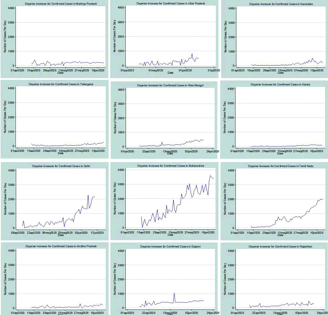
Figure 10: Day wise increase in confirmed cases in 12 different states of India as on June 15, 2020.

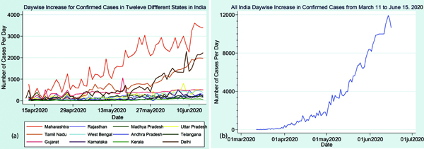
Figure 11: (a) Day- wise increase of confirmed cases in all 12 states in single graph. (b) Day- wise increase of confirmed cases in India.

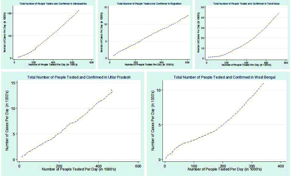
Figure 12: The graph for confirmed cases and samples tested in few states.

Tested samples in few states

The graph for number of people tested was obtained on daily update taken from Indian Council of Medical Research (ICMR) website. The total number of samples tested as on June 15, 2020 in India in different states i.e, TN (729002), MH (671348), RJ (609296) and AP (567375) against the confirmed cases in TN (44661), MH (107958), RJ (12694) and AP (6163). It was observed that few states have very less number of testing labs with which the cases are unknown.

Lockdown period graphs in India

The lockdown period (Figure 13) in all India is divided into four phases initially; later fifth phase named as unlock period (Figure 14) is announced. The first phase was from March 25 to April 14, 2020; the second phase was from April 15 to May 3, 2020. During this lockdown period entire country observed no movement outside the home- ‘Stay Home Stay Safe’ was the quotes referred. The third phase started from May 4 to May 17, 2020 (only 14 days) but the lockdown was extended as the fourth lockdown phase from May 18 to May 31, 2020. After the fourth lockdown, few working sectors and malls were opened with strict guidelines of social distancing and frequently sanitizing to prevent COVID-19 attack. From June 1 to June 31, 2020 was stated as fifth lockdown period in the containment zones. Yet, public transport is not in move.

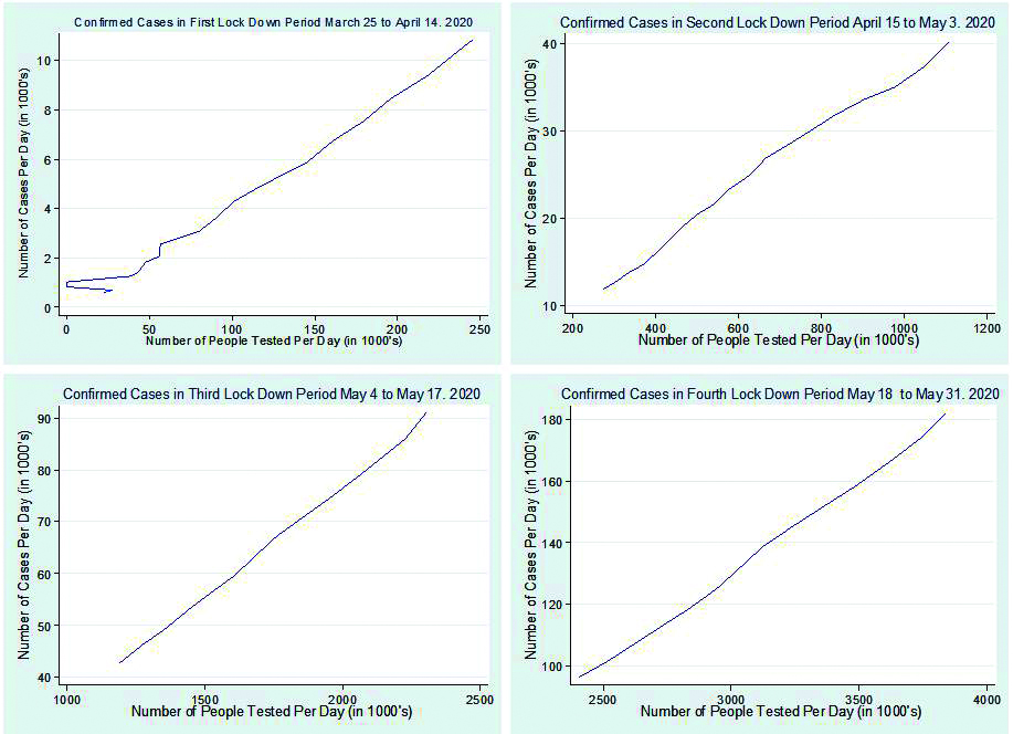
Figure 13: Confirmed cases in four lockdown period in India.

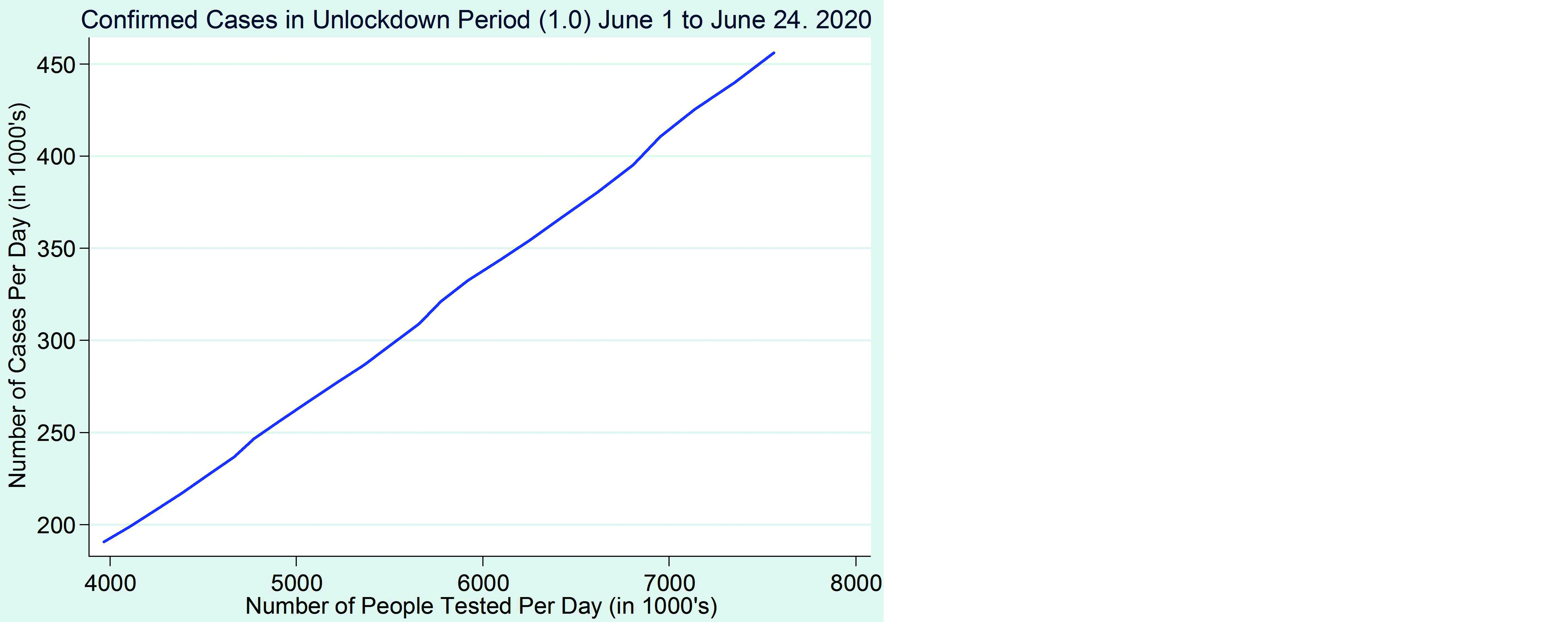
Figure 14: Confirmed cases in unlock down period in India.

Based on the graphs obtained the slope is calculated as in Table 13. The percentage for each slope is obtained as m1 (-5.714 %), m2 (39.393%), m3 (6.521%) and m4 (46.938%).

Table 13: Slope in each lockdown period.

Based on the research work carried out by Mollalo et al. on US continental state where GWR and MGWR were proposed for COVID-19 data of US along with SLM, SEM and OLS models. This study extends its models for three different models of OLS, GLR and GWR with three different cases in each model. In this work, the explanatory were confirmed cases of different weeks of COVID-19 whereas Mollalo et al. modelled on explanatory variables of household income, nursing practioners, number of hospitals and soon. The predict values are mentioned in this work along with the day-wise increase and number of people tested in few states. The lockdown graph with the slope is the highlight of this study (Figure 15).

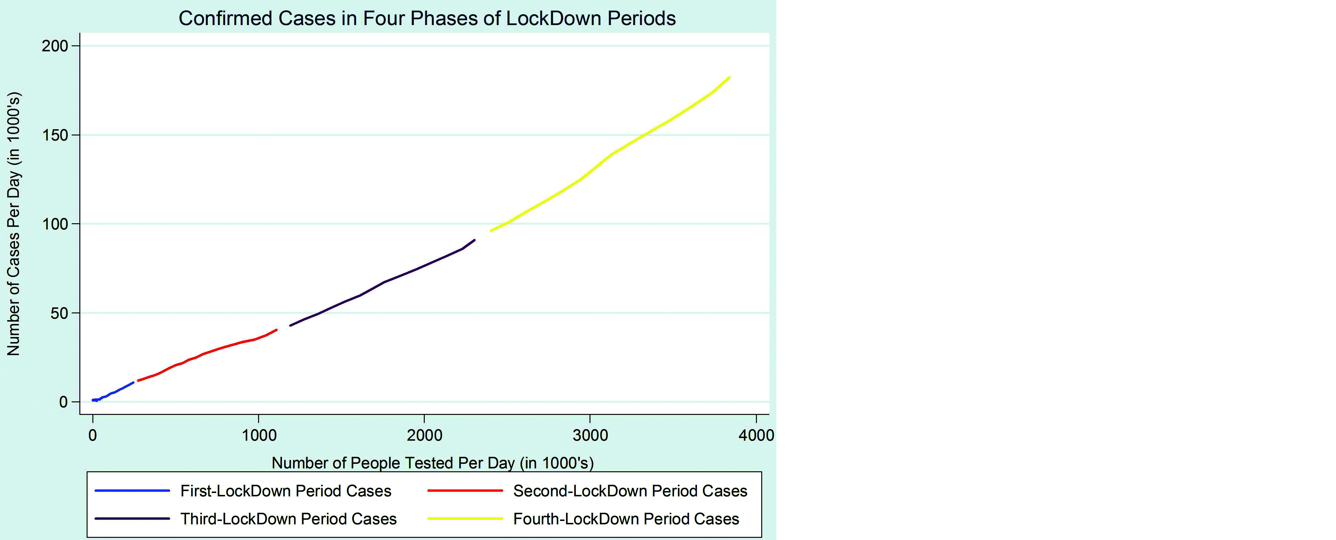
Figure 15: All lockdown period in a single graph.

4. Conclusion

GWR model achieved the highest goodness-of-fit among OLS and GLR models, the results of confirmed cases and the findings of the study proved. GWR obtained AICc (618.9038) and Adj-R² (0.9974) whereas GLR achieved AICc (81132) and Adj-R² (0.0034) and OLS produced AICc (641.1929) and Adj-R2 (0.9941). As stated earlier in discussion since GWR model is a local model compared to GLR and OLS which are global. However, the spatial variability of GWR or OLS or GLR in different countries may reflect different behavior of COVID-19 cases in response to the selected explanatory variables. This study will help in taking the decision for arranging well- equipment testing labs in less availability of testing labs in states of India.

Conflicts of interest

Authors declare no conflicts of interest.

Abbreviations

AICc: Akaike's Information Criterion; DF: Degree of Freedom; SE: Standard Error; VIF: Variance Inflation Factor; OLS: ordinary least models, SLM: spatial lag model; SEM: spatial error model; PLS: Partial Least Square

References

[1] Bashir MF, Ma B, Komal B, Bashir MA, Tan D, et al.Correlation between climate indicators and COVID-19 pandemic in New York, USA. Sci Total Environ. 2020; 728:138835.
[2] WHO. Water, sanitation, hygiene and waste management for the COVID-19 virus. 2020. Available from: https://apps.who.int/iris/handle/10665/331499
[3] Holshue ML, DeBolt C, Lindquist S, Lofy KH, Wiesman J, et al. First case of 2019 novel coronavirus in the United States. The New England Journal of Medicine. 2020; 382:929–936.
[4] Mollalo A, Vahedi B, Rivera KM. GIS-based spatial modeling of COVID-19 incidence rate in the continental United States. Sci Total Environ. 2020; 728:1–8.
[5] Wang C, Zhang J, Yan X, 2012. The Use of Geographically Weighted Regression for the Relationship among Extreme Climate Indices in China. Mathematical Problems in Engineering. Hindawi Publishing Corporation. 2012; 4:1–15.
[6] Calvo E, Escolar M. The Local Voter: A Geographically Weighted Approach to Ecological Inference. American Journal of Political Science. Wiley. 2003; 47(1):189–204.
[7] Comber A, Chi K, Huy MQ, Nguyen Q, Lu B, et al. Distance metric choice can both reduce and induce collinearity in geographically weighted regression. Environment and Planning B: Urban Analytics and City Science. Sage Journal. 2018; 47(3):489–507.
[8] Franch-Pardo I, Napoletano BM, Rosete-Verges F, Billa L. Spatial analysis and GIS in the study of COVID-19. A review. Sci Total Environ. 2020; 739:140033.
[9] Gupta A, Banerjee S, Das S. Significance of geographical factors to the COVID‑19 outbreak in India. Model Earth Syst Environ. 2020; 1–9.
[10] Boulos MNK, Geraghty EM. Geographical tracking and mapping of coronavirus disease COVID‑19/severe acute respiratory syndrome coronavirus 2 (SARS‑CoV‑2) epidemic and associated events around the world: how 21st century GIS technologies are supporting the global fight against outbreaks and epidemics. Int J Health Geogr. 2020 Mar 11;19(1):8.
[11] Krishnakumar B, Rana S. COVID 19 in INDIA: Strategies to combat from combination threat of life and livelihood. J Microbiol Immunol Infect. 2020; 53(3):389–391.
[12] Pulla P. Covid-19: India imposes lockdown for 21 days and cases rise. BMJ. 2020; 368:m1251.
[13] Ward MD, Gleditsch KS. Spatial regression models. Sage Publications. 2018; 155:1–128. ISBN: 9781544328836.
[14] Biuand RS. Regression modeling with spatial dependence: an application of some class selection and estimation methods. Geographical Analysis. 1984; 16(1):25–37.
[15] Srinivasan S. Spatial regression models. Encyclopedia of GIS, Springer International Publishing Switzerland, 2016; 1–6.
[16] Anselin L, Arribas-Bel D. Spatial fixed effects and spatial dependence in a single cross-section. Papers in Regional Science. 2013; 92(1):3–17.
[17] Mogaji KA, Lim HS. A GIS‑based linear regression modeling approach to assess the impact of geologic rock types on groundwater recharge and its hydrological implication. Model Earth Syst Environ. 2019; 6:183–199.
[18] Oshan TM, Smith JP, Fotheringham AS. Targeting the spatial context of obesity determinants via multiscale geographically weighted regression. Int J Health Geogr. 2020; 19(1):1–17.