Full Text

Introduction

Magnetic susceptibility is a physical quantity that indicates the degree of magnetization of an object when exposed to an external magnetic field. Assessment of magnetic susceptibility can be accomplished using quantitative susceptibility mapping (QSM), based on extracting the spatial tissue susceptibility distribution from the measured magnetic resonance imaging (MRI) phase by solving an inverse problem [1]. Development is further spurred by the introduction of ultra-high-field MRI and the associated increase in sensitivity to magnetic susceptibility differences [2].

The QSM technique is being evaluated in a growing number of physiological processes related to brain development and aging, as well as conditions and disease processes such as demyelination, microbleeds, inflammation and iron overload in the brain [3]. In vivo quantification of iron levels may serve as a novel biomarker for diagnosing preclinical Alzheimer’s disease, elevated iron concentration in substantia nigra is associated with Parkinson’s disease, and multiple sclerosis is associated with demyelination and increased iron deposition in deep grey matter [1, 4].

Additionally, the sensitivity to deoxyhemoglobin (dHb) and venous oxygen saturation makes QSM a suitable technique to non-invasively assess brain oxygen extraction and to support studies of cerebral oxygen metabolism. In several diseases, the venous oxygen saturation and oxygen extraction fraction (OEF) is altered, and venous oxygen imaging could serve as an important biomarker associated with disturbed oxygen supply [1, 4, 5].

A dynamic contrast-enhanced QSM-based approach for measurement of perfusion has also been proposed, analogous to dynamic susceptibility contrast MRI (DSC-MRI). Because the magnetic susceptibility is linearly related to contrast-agent (CA) concentration, QSM-based quantification is, in principle, feasible by dynamic measurements of the induced susceptibility shifts in combination with knowledge of the molar susceptibility of the CA [6-8].

The QSM reconstruction process is, however, mathematically challenging and still not fully robust [2, 5]. Critical issues include acquisition of high-quality phase data, lack of signal from surrounding air, phase data post-processing and QSM reconstruction [9]. At the current stage, validations and systematic comparisons are required to allow further progression towards clinical implementation.

Originally, this study aimed at investigating the impact of lack of MRI signal and phase information from surrounding air, by introducing a surrounding aqueous solution with air-equivalent magnetic susceptibility, prepared by doping water with strongly paramagnetic Ho(III)-ions. Holmium has, in this context, the advantage of having only a limited impact on the MR relaxation times. QSM reconstruction is, however, challenging when large susceptibility differences between compartments are present. Hence, this report presents observations made by use of simulations and pilot phantom experiments at 7 T, in connection with QSM reconstruction challenges related to large susceptibility differences and positions near boundaries.

Methods

Theory of quantitative susceptibility mapping

In the brain, the most abundant molecule is water, showing negative volume susceptibility (χ_water=-9.032 ppm) (SI-units). The presence of paramagnetic or diamagnetic substances will affect the susceptibility so that χ_total=χ_water+Δχ. However, since regional susceptibility variations among brain tissues are generally small (±0.1 ppm), brain tissue is still overall diamagnetic. Tissue-specific variations of magnetic susceptibility will disturb the homogeneity of the static magnetic field in an MRI scanner and produce a non-local magnetic field perturbation. The manifested phase change, Δϕ(r), at a given location r, caused by the underlying spatial susceptibility distribution, χ(r), can be expressed as follows [4, 10, 11]:

which, in a k-space representation, is equivalent to:

where r is the position in spherical coordinates, γ is the proton gyromagnetic ratio, B₀ is the magnetic flux density of the main magnetic field, TE is the echo time, 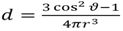is the unit dipole kernel (ϑ) is the observation angle relative the main magnetic field), k_z is the z-component of the k-space vector parallel to the main magnetic field and 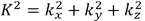is the squared magnitude of the k-space vector. Accurate reconstruction of a susceptibility map relies upon several post-processing steps, briefly outlined below:

Phase unwrapping: Phase aliasing occurs if the true phase exceeds |π|, and this is referred to as phase wraps. Unwrapping algorithms include, for example, path-based [12] or Laplacian-based algorithms [13]. In the former, a path-tracking algorithm is used, comparing phase values of adjacent voxels, and an integer multiplied by 2π is added if the difference between the voxels is larger than π.

Generation of a brain mask: A binary mask is defined to include the susceptibility sources of interest and remove noisy background regions in the phase images. The selection of an appropriate brain mask can be challenging in boundary regions associated with large differences in susceptibility, for example, the air-tissue and tissue-bone interfaces, due to potential signal loss in the magnitude image [4]. Different approaches aiming to achieve accurate brain/non-brain segmentation exist, for example, manual segmentation, surface-model-based, and thresholding-with-morphology [14].

Background field removal: Elimination of background components related to, for example, static magnetic field inhomogeneity, global geometry air-tissue effects and bone interface effects is required for accurate extraction of the local magnetic field induced by the local susceptibility distribution. Imprecise separation of background field and local tissue field may result in uncertainties in regions where a significant variation in susceptibility is present [9]. Two common examples of background removal techniques to address this issue are projection onto dipole fields (PDF) [15] and Laplacian boundary value (LBV) [16].

Field-to-susceptibility inversion: The inversion required to obtain the spatial susceptibility distribution from measured phase is ill-posed (Eq. 2). The dipole kernel is zero at two conical surfaces in k-space defined by  (i.e. corresponding to positions at the magic angle ≈ 54.7^∘ relative the z-direction). At each location on this surface, the susceptibility distribution in k-space can be arbitrarily changed while still producing the same magnetic field [17]. If this issue is not properly addressed in the inversion, the reconstructed susceptibility map will be affected by substantial amplification of small noise contributions and suffer from severe streaking artifacts [18]. Iterative methods, often in combination with some prior information, have been developed. One well-established example is the readily available morphology-enabled dipole inversion (MEDI) algorithm [10, 19]. This algorithm takes advantage of a morphological prior and structural consistency between the magnitude image and the susceptibility map, assuming that edges in the susceptibility map should follow the morphological boundaries. A solution to Eq. 2 is found by using numerical methods to solve a minimization problem of the cost function E [10]:

where M is a structural weighting matrix derived from the magnitude image and used to define edges in the magnitude image, G is the gradient operator, W is a weighting matrix accounting for noise variations over the image, D is the dipole field kernel in k-space, b is the measured local magnetic field and ε is the noise level estimated from the magnitude images. Hence, the first term serves to minimize the edges in the susceptibility map that are not co-localized in the magnitude map, and the second term serves to minimize the difference between the theoretically created magnetic field and the measured magnetic field. The factor λ is the regularization parameter expressing the prioritization between the phase and magnitude information. Setting λ too low in the MEDI algorithm yields an excessively smoothed susceptibility distribution that may prohibit quantification, while too high a λ value will generate maps affected by increased noisiness and streaking artefacts [18].

QSM reconstruction challenges in regions near boundaries are, for example, related to the removal of background field contributions in cases of large susceptibility differences and to the lack of phase information outside the object due to the fact that air does not generate any detectable MR signal [9, 20].

Holmium phantom preparation

With the initial aim to investigate the impact of lack of phase information from the air, an air-equivalent aqueous solution was prepared by doping water with strongly paramagnetic Ho(III) ions. Assuming only a low concentration of a paramagnetic substance, a theoretical volume susceptibility, χ_Ho, of a binary mixture solution of water and Ho(III) can be calculated through Wiedemann’s additivity law [21]. With χ_water=-9.032 ppm and χ_Ho(III) =20715 ppm being the volume susceptibilities of water and the paramagnetic substance Ho(III), respectively, an air-equivalent susceptibility of the holmium aqueous solution, i.e., χ_Ho,air=0.36 ppm, is predicted for the concentration c_Ho,air = 16.96 mM.

The volume susceptibility of a Ho(III)-doped aqueous solution can be experimentally determined by the so-called f₀ method [22]. If the resonance frequency f of a cylinder filled with the solution is measured with the cylinder axis positioned both parallel (//) and perpendicular (^) to the external field, the susceptibility for c=c_Ho can be derived according to:

The susceptibility of the solution is matched to air when f// equals f^. Having this holmium solution surrounding an investigated object would, in principle, allow for analysis related to the missed-out phase information from air, and it would also enable analysis related to reconstruction of large susceptibility differences.

Phantom design

Part 1: Preparation of a holmium solution with air-equivalent susceptibility, to use as a surrounding signal-generating substitute for air. A phantom (Figure 1a), offering a 90° cylinder rotation, was designed to enable experimental determination of an air-equivalent holmium substance according the f₀ method, similar to the approach described by Bakker and de Roos [21]. Five cylinders (Ø 33mm, length 170 mm) were prepared with aqueous holmium solutions containing a gradually increased amount of paramagnetic Ho(III) ions (holmium(III) chloride hexahydrate, 99.9%, Sigma-Aldrich Sweden AB, Stockholm, Sweden), corresponding to a range of molar concentrations c_Ho between 15.5 mM and 18.5 mM.

Part 2: Design of a phantom with the aim to conceptually mimic a central vessel and a vessel near the skull surface, and to scan the phantom to investigate position- and angle-related differences when the object is surrounded by normal air (Figure 1b). Two plastic tubes (Ø 5 mm) with gadolinium (Gd) CA (Dotarem, Guerbet, Paris, France) were placed in a central part and in the bottom part of a water-filled cylinder (Ø 74 mm, length 95 mm),, aiming to mimic a central vessel and a vessel located close to skull surface, respectively, and prepared with three different concentrations of Gd, i.e. 0.05 mM, 1.5 mM and 3 mM. The employed concentrations were selected to approximate susceptibility values of arterial blood, venous blood and blood in presence of Gd CA after intravenous injection, respectively.

Part 3: Design of an extended phantom (Figure 1c), consisting of the water-filled cylinder with the Gd-filled tubes (see Part 2) emerged into a larger cylinder (Ø 153 mm, length 138 mm) filled with the air-equivalent holmium solution prepared according to Part 1. Data from this phantom enables, in principle, a comparison between results with and without phase information from surrounding air, and it also reveals possible reconstruction challenges related to the large susceptibility differences introduced.

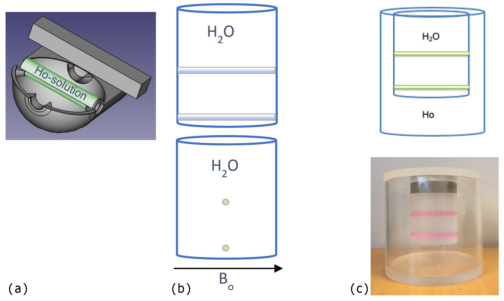
Figure 1: (a) FreeCad drawing of the phantom used to determine an air-equivalent holmium solution. (b) The phantom design aiming to mimic a central vessel and a vessel located close to skull surface, visualized with tubes parallel (top) and perpendicular (bottom) to the main magnetic field B₀. (c) The phantom design consisting of the phantom in (b) emerged in an air-equivalent holmium solution (top) and a corresponding photograph of the phantom (bottom).

Experiments and simulations

Part 1: Each cylinder was scanned at 7 T (Achieva, Philips Healthcare, Best, NL), using multi-echo gradient-echo (GRE) imaging (ΔTE=3.25 ms, matrix 192×192, FOV=180×180 mm²), with the axis of the cylinder parallel with as well as perpendicular to the external field B₀. By use of the obtained phase information, the molar concentration of the holmium-solution corresponding to an air-equivalent solution could be determined according to Eq. 4.

Parts 2 and 3: The phantoms with Gd-filled tubes (Figure 1b-c) were scanned at 7 T, using multi-echo GRE (ΔTE=1.05 ms, matrix 192×192, FOV=180×180 mm2), with the tubes positioned parallel with as well as perpendicular to the main magnetic field, to allow for investigations of angle-related challenges. Obtained phase and magnitude data were used in combination with the MEDI software package. The QSM reconstruction procedures included path-based unwrapping followed by a removal of the background field using the PDF method.

Part 4: Simulations of the complete phantom (corresponding to Figure 1c) were accomplished by calculating phase from simulated susceptibility distributions according to Eq. 1. Subsequent QSM reconstruction performance could then be studied under stable and controlled conditions. A path-based unwrapping was performed followed by removal of the background field using either PDF or LBV. QSM maps were obtained for varying susceptibility differences between the outer compartment (originally designed to contain the holmium) and the inner water compartment with Gd-filled cylinders. The assigned susceptibilities were as follows: χ_H20=-9.032 ppm, χ_Gd-cyl=-8.706 ppm, χ_outer, ranging between -8.5 and 0.36 ppm. The external magnetic field was set parallel with the Gd cylinders. Information, in simulated data, related to the susceptibility difference between the outer compartment and the water compartment was retrieved from ROIs at two different spatial positions of the phantom, i.e. at the level of the bottom tube and the level of the central tube, and as mean values of entire segmented compartments.

In Parts 2-4, QSM estimates were retrieved for (i) a position close to a boundary (allowing study of large susceptibility differences and lack of nearby phase information), and (ii) a central position in the object.

Results

Part 1: The phase information obtained from the five holmium-filled cylinders in the phantom (Figure 1a) was used to calculate the required frequencies and to determine the susceptibility of the solutions according to Eq. 4. The results of the susceptibility values for the different concentrations of Ho(III) ions were plotted in order to determine the holmium concentration corresponding to an air-equivalent solution (Figure 2). The experimental results indicated an air-equivalent susceptibility at a concentration of approximately 16.4 mM Ho(III), in reasonable agreement with the theoretical prediction by Wiedemann’s law.

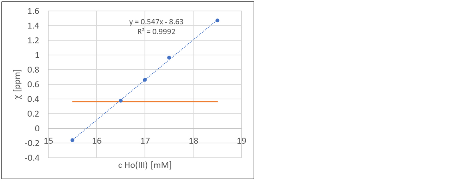
Figure 2: Estimated susceptibilities according to Eq. 4 when using cylinders with different holmium concentrations (blue), and the susceptibility of air (orange horizontal line).

Part 2: Reconstructed QSM images, using the MEDI software package, of the water cylinder with the Gd-filled tubes were assessed by visual inspection, and the susceptibility difference between the Gd-filled tubes and the water was measured for the two differently positioned tubes (i.e., the central and peripheral) in the parallel as well as the perpendicular case.

Pronounced hypointense regions in the vicinity of the bottom tube positioned parallel with the main magnetic field (Figure 3) could be noticed in the QSM maps for all Gd concentrations. For parallel positioning of the tubes in the scanner, the measured susceptibility difference agreed well with the theoretical values for the central tube, but displayed a large deviation for the bottom tube, representing the position close to the boundary (Figure 4, top row). The corresponding measurements in the perpendicular positioning showed, somewhat unexpectedly, less variation between the central and the bottom tube (Figure 4, bottom row).

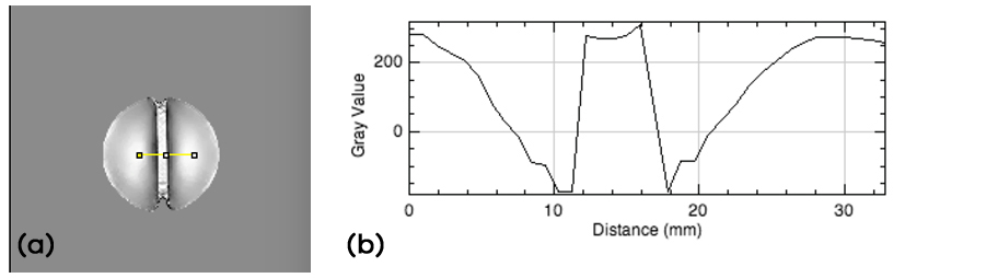
Figure 3: (a) QSM map of peripheral tube position (1.5 mM Gd), parallel with B0. Hypointense areas in the vicinity of the Gd-filled tube can be observed. (b) QSM data (arbitrary units) along the profile indicated in yellow in the QSM map.

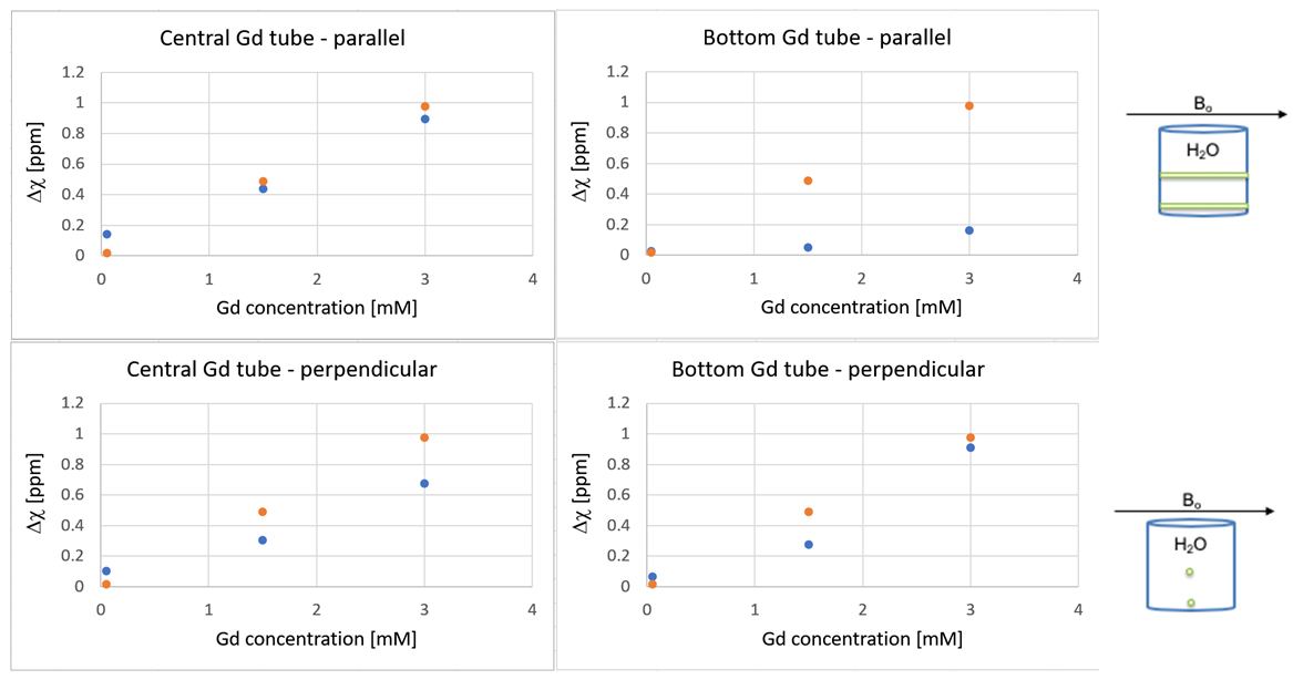
Figure 4: Top row: The theoretical (orange) and the measured (blue) susceptibility difference between the water and the central Gd-filled tube (graph to the left) and the bottom Gd-filled tube (graph to the right), with the tubes positioned parallel with the external magnetic field. Bottom row: The theoretical (orange) and the measured (blue) susceptibility difference between the water and the central Gd-filled tube (graph to the left) and the bottom Gd-filled tube (graph to the right), with the tubes positioned perpendicular to the external magnetic field.

Part 3: Obtained phase and magnitude images from the complete phantom, with the outer holmium cylinder, were processed by use of the MEDI software package, similarly to Part 2. Artefacts and a substantial amount of phase wraps were observed in acquired data (Figure 5), which severely hampered the QSM reconstruction. Major difficulties were encountered in the required post-processing steps, even though different unwrapping algorithms and methods to remove the background field were employed in attempts to reconstruct the susceptibility map, and a deeper understanding of these observations was judged to require supplemental simulations.

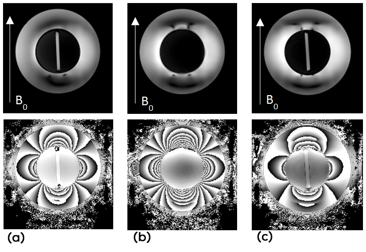
Figure 5: Images of 7 T magnitude (top row) and phase (bottom row) data from positions corresponding to (a) the central Gd-filled tube, (b) in-between the two tubes and (c) the bottom Gd-filled tube in the complete holmium phantom (Figure 1c).

Part 4: In the simulations of the phantom in Figure 1c, the path-based unwrapping process was problematic but possible to handle by manual unwrapping in failed regions. The visual inspection of the reconstructed QSM images from simulated data revealed an increased trend of inverted contrast and streaking artefacts as the susceptibility difference between the outer cylinder and the inner water cylinder, Δχ_outer,H2O (ppm), increased (Figure 6). The Gd-tube positioned in the centre of the water cylinder displayed, generally, a larger internal inhomogeneity compared to the Gd-filled tube positioned at the bottom of the water cylinder. Reconstructed susceptibility differences together with the theoretical difference are shown in Figure 7. The chosen field-removal algorithm also influenced the result. The performance of PDF showed a larger difference between the central and the bottom tube compared with LBV.  

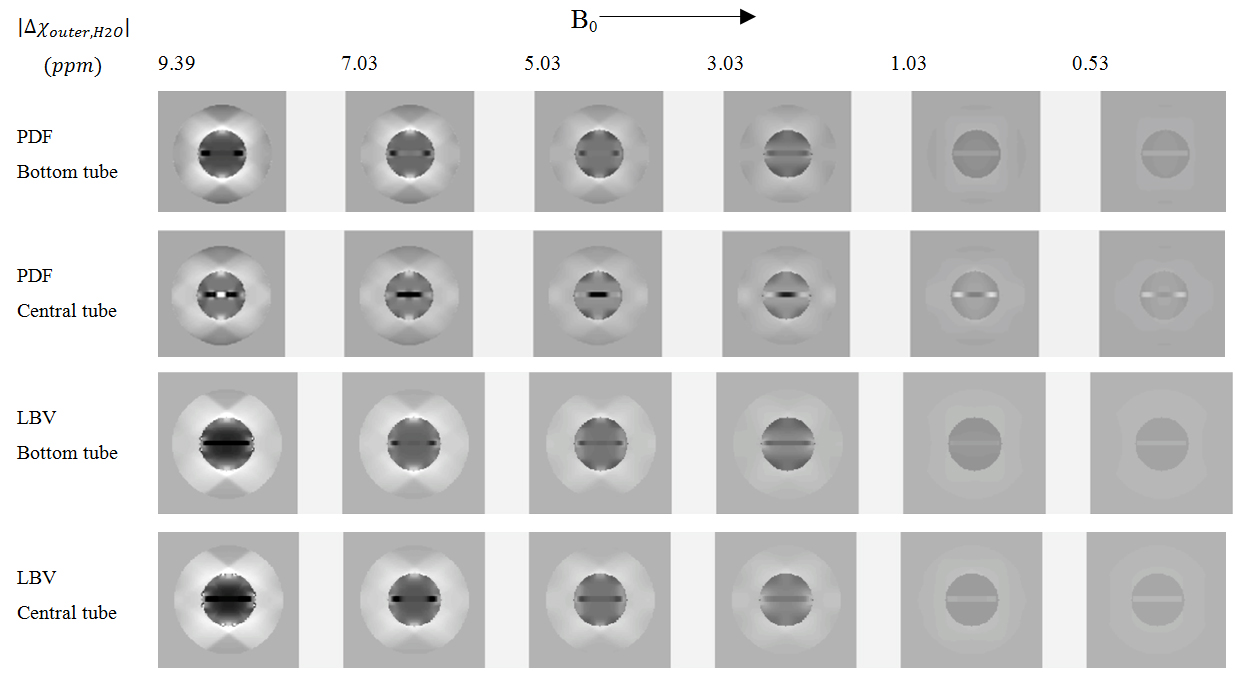
Figure 6: Reconstructed QSM images at two different spatial positions in the simulated complete phantom (Figure 1c), with a decreasing susceptibility difference between the outer cylinder and the inner water-filled cylinder, obtained using PDF (top row) and LBV (bottom row) for removal of the background field.

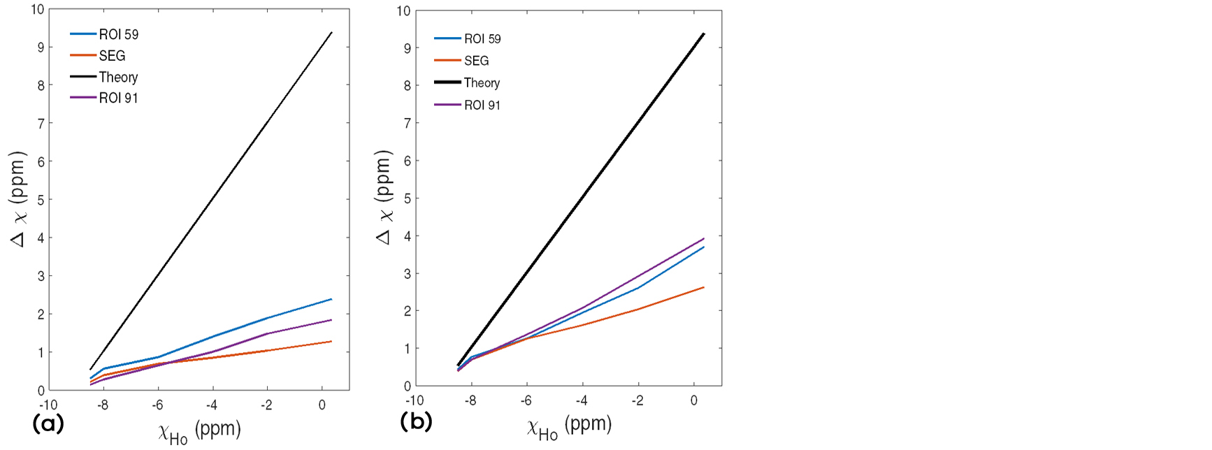
Figure 7: Theoretical (black line) and measured absolute susceptibility differences (in simulated reconstructed data) between the outer compartment and the water compartment as a function of the susceptibility of the outer compartment (χ_Ho) based on (i) ROIs at two different spatial positions of the phantom, i.e. at the level of the bottom tube (blue line, ROI 59) and at the level of the central tube (purple line, ROI 91), and (ii) segmented compartments (red line, SEG), when using PDF (left) and LBV (right) in the post-processing of the QSM reconstruction.

A modest general improvement could be associated with LBV compared to PDF. However, a large discrepancy was revealed for both algorithms as the susceptibility difference between the two compartments was increased, indicating substantial difficulties in MEDI QSM reconstruction of large susceptibility differences. As the theoretical susceptibility difference increased, an extensive underestimation of measured values was noticed. For PDF, slightly improved results were obtained for the bottom tube, compared with the central tube, in agreement with the visual impression of the reconstructed images in Figure 6.

Discussion

One aim of this investigation was to bring renewed attention to the use of a holmium solution with air-equivalent magnetic susceptibility in MRI [21]. The use of a surrounding material able to generate MRI signal, while at the same time exhibiting air-equivalent magnetic susceptibility, might shed further light on challenges and strategies in the design of accurate QSM reconstruction algorithms related to the lack of information from air under normal circumstances. A surrounding material with well-defined magnetic susceptibility would also, in general terms, help evaluating potential QSM reconstruction challenges in regions near boundaries, and by varying the Ho(III) concentration, solutions with a large range of magnetic susceptibilities are achievable.

The QSM concept does not return a global absolute level of magnetic susceptibility, and internal reference regions for quantification can be very difficult to identify, for example, in dynamic studies with CA [23]. Hence, development of reliable external reference structures is warranted, and the introduction of a surrounding, outer, compartment may provide initial insights in how to optimally design such a reference. The accuracy of concentration quantification of CA relies upon the ability to reconstruct the associated (relatively high) CA-induced susceptibility in blood. Hence, as an initial attempt of evaluation, one of the Gd-filled tubes was prepared to represent an approximate susceptibility value of blood in the presence of Gd CA (3 mM), with positions representing a superficial (e.g., the superior sagittal sinus) and an internally located vessel.

Results related to the positioning and orientation of the Gd-filled tubes were intriguing; the slightly improved result obtained (for PDF) in the bottom tube, positioned close to the boundary, compared with the central tube was somewhat unexpected (Figure 7), as was also the improved result for the perpendicular orientation relative to B₀ of the bottom Gd tube in Figure 4. Furthermore, in spite of substantial systematic efforts, difficulties to obtain qualitatively as well as quantitatively reasonable QSM maps remained in cases of large susceptibility differences. The observation of inverted contrast between the Gd-filled tubes and the water is a potential further area of investigation, also related to the behaviour in the vicinity of large susceptibility differences.

We are well aware that the present observations represent particularly challenging conditions in phantoms, of limited importance in daily clinical use. However, it is reasonable for the MRI community to be aware of complicating factors as well as the limits of accurate QSM reconstruction using common and readily available algorithms.

In conclusion, QSM reconstruction still suffers from limited robustness, and this exploratory study demonstrates that details in the mathematical implementation, for example, background field removal, can strongly influence the result. The simulated results were interesting, and awareness with regard to limitations in accuracy of the reconstruction technique could be of importance when large susceptibility differences are to be expected.

Acknowledgements

This study was funded in part by the Swedish Research Council, grant no. MH-2017-0995, and the Swedish Brain Foundation, grant no. FO2018-0145.

Conflict of interest

The authors have no conflicts of interest to disclose.

References

[1] Liu C, Wei H, Gong NJ, Cronin M, Dibb R, et al. Quantitative susceptibility mapping: Contrast mechanisms and clinical applications. Tomography. 2015; 1(1):3–17.
[2] Deistung A, Schweser F, Reichenbach JR. Overview of quantitative susceptibility mapping. NMR Biomed. 2017; 30(4):e3569.
[3] Eskreis-Winkler S, Zhang Y, Zhang J, Liu Z, Dimov A, et al. The clinical utility of QSM: disease diagnosis, medical management, and surgical planning. NMR Biomed. 2017; 30(4):e3668.
[4] Vinayagamani S, Sheelakumari R, Sabarish S, Senthilvelan S, Ros R, et al. Quantitative susceptibility mapping: Technical considerations and clinical applications in neuroimaging. J Magn Reson Imaging. 2021; 53(1):23–37.
[5] Christen T, Bolar DS, Zaharchuk G. Imaging brain oxygenation with MRI using blood oxygenation approaches: methods, validation, and clinical applications. AJNR Am J Neuroradiol. 2013; 34(6):1113–1123.
[6] Lind E, Knutsson L, Ståhlberg F, Wirestam R. Dynamic contrast-enhanced QSM for perfusion imaging: a systematic comparison of ΔR2*- and QSM-based contrast agent concentration time curves in blood and tissue. MAGMA. 2020; 33(5):663–676.
[7] Bonekamp D, Barker PB, Leigh R, van Zijl PC, Li X. Susceptibility-based analysis of dynamic gadolinium bolus perfusion MRI. Magn Reson Med. 2015; 73(2):544–554.
[8] Xu B, Spincemaille P, Liu T, Prince MR, Dutruel S, et al. Quantification of cerebral perfusion using dynamic quantitative susceptibility mapping. Magn Reson Med. 2015; 73(4):1540–1548.
[9] Wang Y, Liu T. Quantitative susceptibility mapping (QSM): Decoding MRI data for a tissue magnetic biomarker. Magn Reson Med. 2015; 73(1):82–101.
[10] Liu J, Liu T, de Rochefort L, Ledoux J, Khalidov I, et al. Morphology enabled dipole inversion for quantitative susceptibility mapping using structural consistency between the magnitude image and the susceptibility map. Neuroimage. 2012; 59(3):2560–2568.
[11] de Rochefort L, Brown R, Prince MR, Wang Y. Quantitative MR susceptibility mapping using piece-wise constant regularized inversion of the magnetic field. Magn Reson Med. 2008; 60(4):1003–1009.
[12] Cusack R, Papadakis N. New robust 3-D phase unwrapping algorithms: application to magnetic field mapping and undistorting echoplanar images. Neuroimage. 2002; 16(3Pt1):754–764.
[13] Schofield MA, Zhu Y. Fast phase unwrapping algorithm for interferometric applications. Opt Lett. 2003; 28(14):1194–1196.
[14] Smith SM. Fast robust automated brain extraction. Hum Brain Mapp. 2002; 17(3):143–155.
[15] Liu T, Khalidov I, de Rochefort L, Spincemaille P, Liu J, et al. A novel background field removal method for MRI using projection onto dipole fields (PDF). NMR Biomed. 2011; 24(9):1129–1136.
[16] Zhou D, Liu T, Spincemaille P, Wang Y. Background field removal by solving the Laplacian boundary value problem. NMR Biomed. 2014; 27(3):312–319.
[17] Haacke EM, Cheng NY, House MJ, Liu Q, Neelavalli J, et al. Imaging iron stores in the brain using magnetic resonance imaging. Magn Reson Imaging. 2005; 23(1):1–25.
[18] Shmueli K, de Zwart JA, van Gelderen P, Li TQ, Dodd SJ, et al. Magnetic susceptibility mapping of brain tissue in vivo using MRI phase data. Magn Reson Med. 2009; 62(6):1510–1522.
[19] Liu T, Liu J, de Rochefort L, Spincemaille P, Khalidov I, et al. Morphology enabled dipole inversion (MEDI) from a single-angle acquisition: comparison with COSMOS in human brain imaging. Magn Reson Med. 2011; 66(3):777–783.
[20] Liu Z, Kee Y, Zhou D, Wang Y, Spincemaille P. Preconditioned total field inversion (TFI) method for quantitative susceptibility mapping. Magn Reson Med. 2017; 78(1):303–315.
[21] Bakker CJ, de Roos R. Concerning the preparation and use of substances with a magnetic susceptibility equal to the magnetic susceptibility of air. Magn Reson Med. 2006; 56(5):1107–1113.
[22] Chu SC, Xu Y, Balschi JA, Springer CS. Bulk magnetic susceptibility shifts in NMR studies of compartmentalized samples: use of paramagnetic reagents. Magn Reson Med. 1990; 13(2):239–262.
[23] Lind E, Knutsson L, Kämpe R, Ståhlberg F, Wirestam R. Assessment of MRI contrast agent concentration by quantitative susceptibility mapping (QSM): application to estimation of cerebral blood volume during steady state. MAGMA. 2017; 30(6):555–566.